From the developer’s website, “Shiny is an R package that makes it easy to build interactive web apps straight from R. You can host standalone apps on a webpage or embed them in R Markdown documents or build dashboards. You can also extend your Shiny apps with CSS themes, htmlwidgets, and JavaScript actions.”
Requirement
Frequently actuaries build summaries of their data to conduct initial data exploration. However this requires many steps including data summarisation in SAS, exporting to Excel, PivotTables and charts. If a factor needs to be changed or adjusted the entire process needs to be repeated. Although tools like Tableau make this much easier to do, shiny is free and is more customisable with the interaction with R packages.
The goal was to create an interactive data explorer that includes the following functionality:
- Dynamic tables and plots for frequency, severity and burning cost
- Automatically define the base value
- Help with factor binning by combining the smallest levels together
- Sort factors in logical order, by exposure size, or the relativity
The model has been updated in August 2021 to address a number of bugs and warnings that appeared in the initial release of the code.
References
Required packages
data.table- Extension ofdata.frameDT- A Wrapper of the JavaScript LibraryDataTablesforcats- Tools for Working with Categorical Variables (Factors)ggplot2- A system for ‘declaratively’ creating graphics, based on “The Grammar of Graphics”haven- Import and ExportSPSS,StataandSASFilesHmisc- Harrell MiscellaneousinsuranceData- A Collection of Insurance Datasets Useful in Risk Classification in Non-life Insuranceplotly- Create Interactive Web Graphics viaplotly.jspurrr- Functional Programming Toolsscales- Scale Functions for Visualizationshiny- Web Application Framework for Rstringi- Character String Processing Facilities
Inputs
The settings below are required to direct the program to the correct data and fields:
dt- Data source which should be adata.table(notdata.frame). There is commented code for importing a SAS dataset using thehavenpackage if required.- In order to make the program more easily transferable
dataCarfrom theinsuranceDatapackage is used. “This data set is based on one-year vehicle insurance policies taken out in 2004 or 2005. There are 67856 policies, of which 4624 (6.8 (sic)”. var_exposure- Specify the field that contains the exposure field.var_claim- Specify the field that contains the number of claims.var_incurred- Specify the field that contains the incurred losses.var_drop- Note any fields to exclude from the review.
There are additional user interface constants however these typically do not need to be modified. They are explained further in the comments.
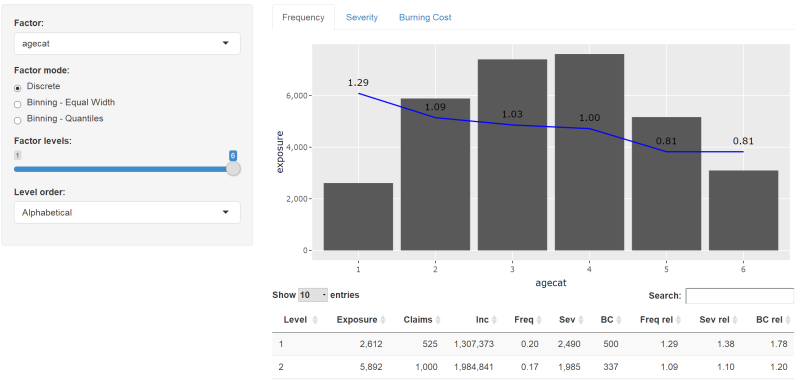
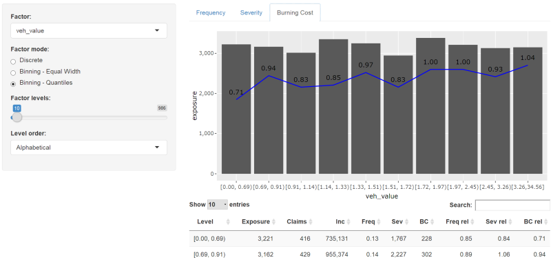
Outputs
Sample screenshots shown below:
Solution
This has been developed on R 4.1.1 and shiny 1.6.0
- Copy the code into a new R script in RStudio
- Save the script
- Click the button ‘Run App’
# Shiny data explorer -----------------------------------------------------
# Simon - actuary.rbind.io
# v2 - updated in 2021-08

# Initial declarations ----------------------------------------------------
library(data.table)
library(DT)
library(forcats)
library(ggplot2)
library(haven)
library(Hmisc)
library(plotly)
library(purrr)
library(scales)
library(shiny)
library(stringi)

# read in data and convert to data.table
library(insuranceData) # for distribution have included sample file
data(dataCar)
dt <- setDT(dataCar)
detach("package:insuranceData", unload=TRUE)
# library(haven) # use haven to read in SAS datasets
# dt <- setDT(read_sas("C:/mtcars.sas7bdat"))

# classify all the variables from the data.table
# note that R is case sensitive
var_list <- names(dt)
var_exposure <- "exposure" # must be defined
var_claim <- "numclaims" # must be defined
var_incurred <- "claimcst0" # must be defined
var_drop <- c("X_OBSTAT_",
              var_list[grep("^delete_all_vars_beginning_with_this_string", var_list, ignore.case = TRUE)],
              var_list[grep("delete_all_vars_ending_with_this_string$", var_list, ignore.case = TRUE)]
)
var_measures <- c(var_exposure, var_claim, var_incurred)
var_analysis <- setdiff(var_list, c(var_drop, var_measures))

# define the names of variables that will be used later
var_prefix <- "_" # used to make the variable more unique in case the source dataframe uses these names
var_freq <- paste0(var_prefix, "Freq")
var_freq_rel <- paste0(var_prefix, "Freq_rel")
var_sev <- paste0(var_prefix, "Sev")
var_sev_rel <- paste0(var_prefix, "Sev_rel")
var_bc <- paste0(var_prefix, "BC")
var_bc_rel <- paste0(var_prefix, "BC_rel")

# user interface constants
selected_fct_mode_choices_character <- c("Discrete")
selected_fct_mode_choices_numeric <- c("Discrete", "Binning - Equal Width", "Binning - Quantiles")
selected_fct_levels_default_max <- 25 # if there are a large number of levels, will default to this number instead of max
fct_level_other <- "Other" # this is the value of the condensed bins in fct_lump
selected_level_order_choices_freq <- c("Level asc","Exposure desc", "Frequency asc")
selected_level_order_choices_sev <- c("Level asc","Claims desc", "Severity asc")
selected_level_order_choices_bc <- c("Level asc","Exposure desc", "Burning Cost asc")

plot_y_rel_nudge_factor <- -0.2 # used to shift the relativity line on the graph
plot_y_rel_label_nudge_factor <- 0.05 # used to shift up the labels on the graph
rel_rounding <- 2 # number of decimal places shown in the relativity chart
datatable_colnames <- c("Level","Exposure","Claims","Inc","Freq","Sev","BC","Freq rel","Sev rel","BC rel") # these are the column names in the Shiny datatable

# Preliminary data processing ---------------------------------------------

# drop the variables in var_drop
if (length(var_drop > 0)) {dt[, c(var_drop) := NULL]}
# apply any custom data adjustments to dt here
#
# summarise the data to speed up results
dt_sum <- dt[, lapply(.SD, sum, na.rm = TRUE), by = c(var_analysis), .SDcols = c(var_measures)]

# Key functions -----------------------------------------------------------

# helper function convert a factor to numeric
factorToNumeric <- function(input_factor){
  return(as.numeric(levels(input_factor))[input_factor])
}

# function that returns a data.table with
# 1) binned factor levels
# 2) statistics summarised at the binned levels
# 3) ratio calculations
summariseData <- function(input_data, input_var, input_fct_mode, input_fct_levels){

  # for the levels analysis can use the summarised dataframe for speed
  # uses fct_lump to allow user to reduce the number of levels
  if (input_fct_mode == "Discrete"){
    # read in the summarised data
    output_data <- input_data[["dt_sum"]][, lapply(.SD, sum,na.rm=TRUE), by = c(input_var), .SDcols = c(var_measures)]
    output_data[, new_var := fct_lump_n(factor(get(input_var), exclude=c()), n = input_fct_levels - 1, w = get(var_exposure), other_level = fct_level_other)]
  }
  # for the binned data analysis need to use the full unsummarised dataframe
  else if (input_fct_mode %in% c("Binning - Equal Width","Binning - Quantiles")){

    # read in the unsummarised data
    output_data <- input_data[["dt"]][, c(input_var, var_measures), with = FALSE]

    # for bins of equal width, define cuts from min(input_var) to max(input_var)
    if (input_fct_mode == "Binning - Equal Width"){
      input_var_min <- min(output_data[[input_var]], na.rm = TRUE)
      input_var_max <- max(output_data[[input_var]], na.rm = TRUE)
      output_data[, new_var := cut2(get(input_var), cuts = seq(input_var_min, input_var_max, (input_var_max-input_var_min)/input_fct_levels), m = 0)]
      # for quantiles, use the number of groups
    } else if (input_fct_mode == "Binning - Quantiles"){
      output_data[, new_var := cut2(get(input_var), g = input_fct_levels, m = 0)]
    }
  }

  # if numeric sort the new_var in ascending order upon the underlying data in input_var
  if (class(output_data[[input_var]]) == "numeric"){
    output_data <- output_data[, c(lapply(.SD, sum, na.rm = TRUE), input_var_mean = mean(get(input_var))), by = new_var, .SDcols = c(var_measures)]
    setorder(output_data, input_var_mean)
    output_data[,input_var_mean:=NULL]
  } else {
    output_data <- output_data[, lapply(.SD, sum, na.rm = TRUE), by = new_var, .SDcols = c(var_measures)]
    setorder(output_data, new_var)
  }
  setnames(output_data, "new_var", input_var)

  # calculate ratios
  output_data[, c(var_freq) := get(var_claim)    / get(var_exposure)]
  output_data[, c(var_sev)  := get(var_incurred) / get(var_claim)   ]
  output_data[, c(var_bc)   := get(var_incurred) / get(var_exposure)]

  # identify the level with the most exposure and determine base relativity (excluding Other and NA levels)
  base_level <- output_data[!(get(input_var) %in% c(fct_level_other, NA)), .SD[which.max(get(var_exposure))]]
  # if discrete with 1 factor level then set the base_level to fct_level_other
  if (input_fct_mode == "Discrete" & input_fct_levels == 1){
    base_level <- output_data[get(input_var) == fct_level_other,]
  }
  base_freq <- base_level[,get(var_freq)]
  base_sev  <- base_level[,get(var_sev)]
  base_bc   <- base_level[,get(var_bc)]

  # add the relativities
  output_data[, c(var_freq_rel) := round(get(var_freq) / eval(base_freq), rel_rounding)]
  output_data[, c(var_sev_rel)  := round(get(var_sev)  / eval(base_sev) , rel_rounding)]
  output_data[, c(var_bc_rel)   := round(get(var_bc)   / eval(base_bc)  , rel_rounding)]

  return(output_data)
}

# reorder the factor levels based upon the user input
orderLevel <- function(input_data, input_var, input_order){

  # adjust the factor levels based upon the user selection
  if (input_order == "Level asc") {

    # establish the appropriate alphabetical sort order
    # if the list does not contain fct_level_other use the data as pre-sorted in summariseData
    # else regular sort with fct_level_other at the end
    sort_order <- levels(input_data[[input_var]])
    if (!has_element(sort_order, fct_level_other)) {
      input_data[, c(input_var) := fct_inorder(factor(get(input_var), exclude=c()))]
    } else {
      sort_order <- c(sort(sort_order[sort_order != fct_level_other]), fct_level_other)
      input_data[, c(input_var) := fct_relevel(factor(get(input_var), exclude=c()), sort_order)]
    }
  } else if (input_order == "Exposure desc") {
    input_data[, c(input_var) := fct_reorder(factor(get(input_var), exclude=c()), get(var_exposure), .desc=TRUE)]
  } else if (input_order == "Claims desc") {
    input_data[, c(input_var) := fct_reorder(factor(get(input_var), exclude=c()), get(var_claim), .desc=TRUE)]
  } else if (input_order == "Frequency asc") {
    input_data[, c(input_var) := fct_reorder(factor(get(input_var), exclude=c()), get(var_freq), .desc=FALSE)]
  } else if (input_order == "Severity asc") {
    input_data[, c(input_var) := fct_reorder(factor(get(input_var), exclude=c()), get(var_sev), .desc=FALSE)]
  } else if (input_order == "Burning Cost asc") {
    input_data[, c(input_var) := fct_reorder(factor(get(input_var), exclude=c()), get(var_bc), .desc=FALSE)]
  }

  # reorder input_data based upon the new level ordering
  input_data <- input_data[order(get(input_var))]
}

# draws a relativity plot
# x-axis containing the categories
# y-axis containing the exposure amount and the level relativities
plotGraph <- function(input_data, input_var, y_data, y_rel) {

  # ggplot2 does not easily support two axis graphs
  # instead will transform y_rel to the y_data basis and label
  # https://stackoverflow.com/questions/3099219/plot-with-2-y-axes-one-y-axis-on-the-left-and-another-y-axis-on-the-right
  # scaling factor is determined based upon the ratio of  max(y_data) and max(y_rel)
  y_data_max <- max(input_data[[y_data]], na.rm = TRUE)
  y_rel_max <- max(input_data[[y_rel]], na.rm = TRUE)
  rel_scale_factor <- (1 + plot_y_rel_nudge_factor) * y_data_max / y_rel_max

  #define the plot object
  p <- ggplot(input_data, aes(x=get(input_var))) +
    geom_col(aes(y=get(y_data))) +
    geom_line(aes(y=get(y_rel) * rel_scale_factor), stat = "identity", group = 1, colour = "blue") +
    geom_text(aes(y=get(y_rel) * rel_scale_factor), stat = "identity", group = 1,
              label = sprintf(paste0("%0.", rel_rounding, "f"), round(input_data[,get(y_rel)], digits = rel_rounding)),
              nudge_y = y_data_max * plot_y_rel_label_nudge_factor) +
    scale_y_continuous(name=y_data, labels = comma) +
    #scale_y_continuous(name=y_data, labels = comma, sec.axis=sec_axis(~./re_scale_factor, name=y_rel)) +
    xlab(input_var) +
    NULL
  return (p)
}

# UI for application ------------------------------------------------------

ui <- fluidPage(

  # Application title
  titlePanel("Shiny data explorer"),

  # Sidebar for all user controls
  sidebarLayout(
    sidebarPanel(
      selectInput(inputId = "selected_fct",
                  label = "Factor mode:",
                  choices = sort(var_analysis)),
      radioButtons(inputId = "selected_fct_mode",
                   label = "Factor mode:",
                   choices = selected_fct_mode_choices_numeric),
      sliderInput(inputId = "selected_fct_levels",
                  label = "Factor levels:",
                  min = 1,
                  max = selected_fct_levels_default_max,
                  value = selected_fct_levels_default_max,
                  step = 1,
                  round = TRUE,
                  ticks = FALSE),
      selectInput(inputId = "selected_level_order",
                  label = "Level order:",
                  choices = selected_level_order_choices_freq)
    ),

    # Show the primary plot
    mainPanel(

      # Output: Tabset w/ plot, summary, and table
      # Use of plotly is optional, can also plot static ggplot2 charts
      tabsetPanel(id = "selected_tab",
                  selected = "Frequency",
                  type = "tabs",
                  tabPanel(title = "Frequency", plotlyOutput("freqPlot")),
                  tabPanel(title = "Severity" , plotlyOutput("sevPlot")),
                  tabPanel(title = "Burning Cost" , plotlyOutput("bcPlot"))
      ),
      DTOutput("tableValues")
    )
  )
)

# Define server logic -----------------------------------------------------

server <- function(input, output, session) {

  # when changing tabs update the level order selections
  observeEvent(eventExpr = input$selected_tab, handlerExpr = {
    if (input$selected_tab == "Frequency") {
      updateSelectInput(session = session, "selected_level_order", choices = selected_level_order_choices_freq)
    } else if (input$selected_tab == "Severity") {
      updateSelectInput(session = session, "selected_level_order", choices = selected_level_order_choices_sev)
    } else if (input$selected_tab == "Burning Cost") {
      updateSelectInput(session = session, "selected_level_order", choices = selected_level_order_choices_bc)
    }
  })

  # when changing factors
  # adjust selected_fct_mode and selected_fct_levels max
  observeEvent(eventExpr = input$selected_fct, handlerExpr = {


    # if this is a character variable only allow discrete factor levels to be chosen
    input_var_class <- class(dt_sum[[input$selected_fct]])
    if (input_var_class == "numeric") {
      updateRadioButtons(session = session, "selected_fct_mode", choices = selected_fct_mode_choices_numeric)
    } else if (input_var_class %in% c("character","factor")) {
      updateRadioButtons(session = session, "selected_fct_mode", choices = selected_fct_mode_choices_character)
    } else {
      updateRadioButtons(session = session, "selected_fct_mode", choices = NULL)
    }

    # update the max(val) of sliderInput
    updateSliderInput(session = session, "selected_fct_levels", max = min(selected_fct_levels(), selected_fct_levels_default_max))
  })

  # define the reactive dataframes
  # these are defined separately as ordering levels does not require recalculation of data_sum()
  selected_fct_levels <- reactive(length(unique(dt_sum[[input$selected_fct]])))
  data_sum <- reactive(summariseData(list(dt_sum = dt_sum,dt = dt), input$selected_fct, input$selected_fct_mode, input$selected_fct_levels))
  data_sum_sort <- reactive(orderLevel(data_sum(), input$selected_fct, input$selected_level_order))

  # output the tabbed plots
  output$freqPlot <- renderPlotly({
    ggplotly(plotGraph(data_sum_sort(), input$selected_fct, var_exposure, var_freq_rel))
  })
  output$sevPlot <- renderPlotly({
    ggplotly(plotGraph(data_sum_sort(), input$selected_fct, var_claim, var_sev_rel))
  })
  output$bcPlot <- renderPlotly({
    ggplotly(plotGraph(data_sum_sort(), input$selected_fct, var_exposure, var_bc_rel))
  })

  # convert data_sum_sort() to a dataframe and render in Shiny
  output$tableValues <- renderDT(
    data_sum_sort() %>%
      datatable (rownames = FALSE, colnames = datatable_colnames) %>%
      formatRound(c(var_measures, var_sev, var_bc), digits = 0) %>%
      formatRound(c(var_freq, var_freq_rel, var_sev_rel, var_bc_rel), digits = rel_rounding) %>%
      identity()
  )
}

# Run the application -----------------------------------------------------

shinyApp(ui = ui, server = server)