Requirement
The glmnet package is an implementation of “Lasso and Elastic-Net Regularized Generalized Linear Models” which applies a regularisation penalty to the model estimates to reduce overfitting. In more practical terms it can be used for automatic feature selection as the non-significant factors will have an estimate of 0. glmnet has built in functionality for log-poisson models which are commonly used by actuaries for frequency and claim count models.
Unlike the glm function in R, glmnet itself does not accept data.frame objects as an input and requires a model matrix. This brief tutorial will show how we can implement a Poisson frequency glmnet in R with a sample insurance dataset.
Suggested references
- An introduction to glmnet
- CAS Monograph No. 5: Generalized Linear Models for Insurance Rating, 2nd Edition
- In-depth introduction to machine learning in 15 hours of expert videos
- See Chapter 6: Linear Model Selection and Regularization
- Using PROC GENMOD to find a fair house insurance rate for the Norwegian market
Required packges
glmnet- Lasso and Elastic-Net Regularized Generalized Linear ModelsMatrix- Sparse and Dense Matrix Classes and MethodsinsuranceData- A Collection of Insurance Datasets Useful in Risk Classification in Non-life Insurance
Notable packages
gamlr- Gamma Lasso RegressionglmnetUtils- Utilities for ‘Glmnet’- Includes some tools to make it easier to work directly with
data.frames, use formulas to define the model structure, and generate model matrices.
- Includes some tools to make it easier to work directly with
Inputs
SingaporeAuto- This is a dataset from theinsuranceDatapackage containing a number of rating factors
Outputs
cvfit- Fitted glm objectplot(cvfit)- Plot the improvement against the target optimisation function, in this case poisson deviancecoef(cvfit, ...)- Estimated coefficientsexp(predict(cvfit, ...))- Predicted claim counts
Testing a conversion of a simple data.frame to a sparse model matrix
This step is optional however provides background to show how to create the model matrix and how it converts a data.frame into a matrix. This is usually required in other machine learning applications. The primary change is that factors or factor-like variables such as characters are one-hot encoded, for example here column a_factor which can be a, b, or c has been converted to a_factora, a_factorb, a_factorc each of which can take a value of 0 or 1. If a numeric variable is not classed as a factor, it will be treated as a numeric value for the model fit, e.g. c_numeric. A sparse matrix is a matrix where the 0 values in the matrix are replaced with a missing value to reduce the object size.
The method used here will use the function sparse.model.matrix. In the code ~. means we will take all the columns within the dataset df and -1 excludes the generated intercept value. This is not required as the glmnet fit will generate an intercept estimate. glmnet versions 3.0+ now include the makeX function which performs a similar function as a wrapper to sparse.model.matrix.
library(Matrix)

# define a simple data.frame
a_factor <- factor(rep(c('a','b','c'), 2))
b_char <- rep(c('d','e','f'), 2)
c_numeric <- c(1:6)
df <- data.frame(a_factor,b_char,c_numeric)

# standard method
sparse.model.matrix(~. -1, df) # ~. include all columns and adds intercept
## 6 x 6 sparse Matrix of class "dgCMatrix"
##   a_factora a_factorb a_factorc b_chare b_charf c_numeric
## 1         1         .         .       .       .         1
## 2         .         1         .       1       .         2
## 3         .         .         1       .       1         3
## 4         1         .         .       .       .         4
## 5         .         1         .       1       .         5
## 6         .         .         1       .       1         6
# glmnet makeX function
library(glmnet)
makeX(df, sparse = TRUE)
## 6 x 7 sparse Matrix of class "dgCMatrix"
##   a_factora a_factorb a_factorc b_chard b_chare b_charf c_numeric
## 1         1         .         .       1       .       .         1
## 2         .         1         .       .       1       .         2
## 3         .         .         1       .       .       1         3
## 4         1         .         .       1       .       .         4
## 5         .         1         .       .       1       .         5
## 6         .         .         1       .       .       1         6
Prepare the data for the model
We create a new data.table called dt_feature which is a cleaned up version of the features we want to include in our model. Note here that data.table is used here as a personal preference, dplyr or data.frame would work as well. For claims count GLMs we also need to create an offset value which acts a scaling multiplier for the earned exposure, i.e. a 1.5 year policy should have 1.5x the predicted claims. Refer the to the reference document for a more detailed explanation on offsets and an example from SAS.
library(data.table) # used as a preference for this example
library(insuranceData)
library(glmnet)
library(Matrix)

# import the data and process the variables for analysis
data(SingaporeAuto)
dt <- setDT(SingaporeAuto)
rm(SingaporeAuto)
dt_feature <- dt[,  .(
                    SexInsured=factor(SexInsured),
                    Female=factor(Female),
                    Private=factor(PC),
                    NCDCat=factor(NCD),
                    AgeCat=factor(AgeCat),
                    VAgeCat=factor(VAgeCat)
                    )]

# create the sparse feature matrix excluding the numeric variables
m_feature <- sparse.model.matrix(~., dt_feature)
m_offset <- log(dt[["Exp_weights"]])
m_counts <- dt[["Clm_Count"]]
Fit glmnet using cross validation
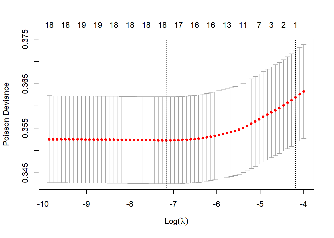
k-fold cross validation splits the data into k parts in order to help test the optimal regularisation factor lambda. There are two lambda values provided by default from the model fit object:
lambda.minthe one that achieves the minimum poisson deviancelambda.1sethe “most regularized model such that error is within one standard error of the minimum” (glmnet).Nonzeroexpresses the number of factor levels that are non-zero (excluding the intercept).
Because the cross validation folds are sampled at random, the results may vary upon each execution of the program. For reproducibility purposes the random number generator seed has been defined.
set.seed(12345) # reproducible random numbers
cvfit = cv.glmnet(m_feature, m_counts, offset = m_offset, family = "poisson")
cvfit
##
## Call:  cv.glmnet(x = m_feature, y = m_counts, offset = m_offset, family = "poisson")
##
## Measure: Poisson Deviance
##
##       Lambda Index Measure       SE Nonzero
## min 0.000775    35  0.3523 0.009777      17
## 1se 0.015221     3  0.3619 0.010464       1
The poisson deviance at each model iteration is shown on the plot.
plot(cvfit)
The model coefficients can be shown as follows for both lambda values.
cbind(coef(cvfit, s = "lambda.1se"), coef(cvfit, s = "lambda.min"))
## 23 x 2 sparse Matrix of class "dgCMatrix"
##                     s1          s1
## (Intercept) -1.9876630 -1.70480890
## (Intercept)  .          .
## SexInsuredM  .          0.09709391
## SexInsuredU  .          .
## Female1      .         -0.02808719
## Private1     .          .
## NCDCat10     .         -0.26573355
## NCDCat20     .         -0.38844888
## NCDCat30     .         -0.28366046
## NCDCat40     .         -0.62968611
## NCDCat50     .         -0.61479835
## AgeCat2      .          .
## AgeCat3      .          0.05642882
## AgeCat4      .          .
## AgeCat5      .         -0.12825621
## AgeCat6      .          0.34274113
## AgeCat7      .          0.41041089
## VAgeCat1     .          0.17485142
## VAgeCat2     .          0.39802069
## VAgeCat3     .          0.13762082
## VAgeCat4     .         -0.22433971
## VAgeCat5    -0.1279539 -0.95229715
## VAgeCat6     .         -1.18753843
The predicted number of claims can be calculated as follows. For brevity only the first 10 are shown using the head function.
head(exp(predict(cvfit, newx = m_feature, newoffset = m_offset, s = "lambda.min")), 10)
##     lambda.min
## 1  0.091457290
## 2  0.077588767
## 3  0.068967793
## 4  0.112736861
## 5  0.066156960
## 6  0.092822266
## 7  0.025219947
## 8  0.031499199
## 9  0.006279252
## 10 0.018940695